This blogpost attempts to give a comprehensive introduction to the framework of the SINDy algorithm, described mainly in the following three papers:

• ‘Discovering Governing Equations from Data by Sparse Identification of Nonlinear Dynamical Systems’ [1]
• ‘Data-Driven Discovery of Coordinates and Governing Equations’ [2]
• ‘Data-Driven Discovery of Partial Differential Equations’. [3]

The work on SINDy and related projects is still very much ongoing and each year numerous breakthroughs are made. Here, I just try to highlight the concept, as well as some of the initial successes that have been achieved.

Discovering governing equations – The need for SINDy

“Not only is the Universe stranger than we think, it is stranger than we can think.” —Werner Heisenberg.

One of the main goals of science is to describe the world in terms of theories, simple ideas and formulas. To discover models that capture the essence of vastly complex systems and give us the power to predict what will happen next, or how we can influence the system to our advantage. In our pursuit of these models, the problems we have tried to tackle have become increasingly harder. Having realized that solving systems analytically is becoming more and more unfeasible, science has made a drastic migration to the computational domain ever since its power became available. For many of the hot topics in science today- climate science, neuroscience, ecology, finance, epidemiology, etc.- data are abundant, but good models remain elusive. As the quote by Heisenberg suggests, maybe some of these systems surpass what we as humans are capable of grasping. Maybe, we need to rely on machines to help us discover models and dynamics. And what better tool to use than machine learning?

Many papers in recent years have described the construction of surrogate models. These are usually neural networks, that use a vast amount of parameters to mimic what the actual, ‘nature informed’ or ‘physics informed’ and human-made models predict. Although this approach is quite promising and has proven already to be of great value in many cases, they remains subject to the largest downside of neural networks; interpretability. The networks find patterns and behaviours that are beyond human comprehension and even though it can handle them personally, it fails to provide the scientist behind the process with an interpretation of how it arrives at the right solution. Sparse Identification of Nonlinear Dynamics on the other hand, or SINDy for short, tries to do exactly this. It builds on the observation that many natural systems are governed by equations containing only a few terms (in an appropriate basis, that is) and tries to implement this into its algorithm. SINDy applies a combination of sparsity-promoting techniques and machine learning to nonlinear dynamical systems to discover governing equations from noisy measurement data. So not only does it learn a model, it does so following our intuition on how nature usually behaves and provides us with an interpretable ‘window’ into the system. In what follows, I will try to walk you through the working principles of SINDy. We’ll explore some of the problems the authors were able to solve, some of the hurdles they overcame and have yet to overcome and some valuable extensions to the framework.

Example- The Lorenz system

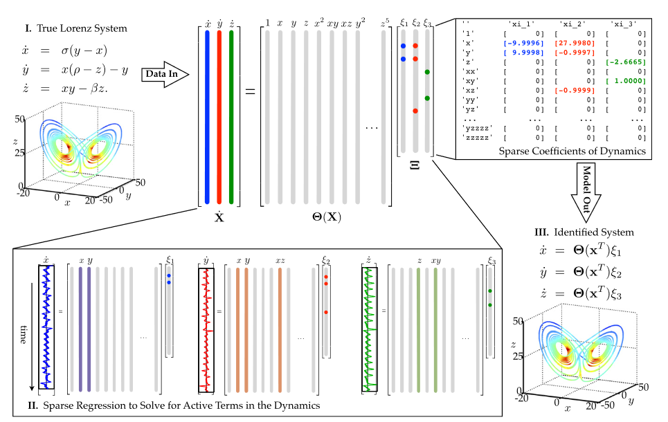
For me, the algorithm is most easily explained by immediately looking at some of the problems it can tackle. As a first example, consider (the Lorenz system). It was introduced in 1963 by Edward Lorenz, Ellen Fetter and Margaret Hamilton as a simplified model for atmospheric convection (and later used as a model for many other physical phenomena). Even though it is quite compact in structure, it was one of the first systems that popularized chaos theory, as the system can display chaotic behaviour under the right initial conditions.

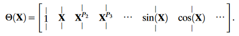
SINDy is used to try and recover this system of coupled equations, based solely on a time history of the ‘state x(t)’ (here x,y,z). The input to the model consists of a time series of this state and its time derivative (either given or computed numerically). With this input, a library $\Theta$(X) is constructed, consisting of all the candidate nonlinear terms built from X we want to include as possible terms. Each one of these terms can then show up in the resulting equations. With P_n denoting polynomial terms of order n, an example library may look like this:

The sparse regression problem that is subsequently solved using standard machine learning techniques, is simply stated as

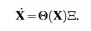
We try to find the sparse set of coefficients given by $\Xi$. This is a sparse matrix, with the nonzero elements indicating what terms from the candidate library should be present in the system of equations. Essentially, for every coordinate of the original problem, a sparse regression has to be solved in this manner. This already highlights one of the major limitations of this model, as a solution quickly becomes unfeasible as the number of coordinates grows.

—‘Discovering Governing Equations from Data by Sparse Identification of Nonlinear Dynamical Systems’ [1]

The model for the Lorenz system is shown schematically above. The function library $\Theta$(X) contains mixed polynomial terms up to order 5 and the $\Xi$ matrix is clearly very sparse, with only a couple of nonzero (coloured) coefficients. Even though the input data are noisy (mainly caused by the numerical errors introduced by taking the time derivative), the true model is retrieved exceptionally well, with all the correct terms being identified, as well as the magnitudes of the coefficients.

Example - Von Karman vortex street

—NASA Worldview

As a second example of the method, the original paper discusses the modelling of fluid flow around a cylinder. For low Reynold’s number (Re~100), the flow organizes into a well known Von Karman vortex street quickly. In principle, the flow field is defined by its value on the whole two-dimensional grid of the simulated test data. As mentioned in the previous section though, this would mean that we have to solve a regression optimization for each individual gridpoint, a task that is unfeasible and highly overcomplicated. In order to tackle the problem more efficiently -and this is an important remark in general for the SINDy method and its alternatives-, we can include prior knowledge we have of the system. We have, after all, in most cases some available information on the system of interest. However strong our computers or models may become, it is the task of a scientist to guide the process.

A very adequate method that can be used here, is the proper orthogonal decomposition or POD (otherwise known as PCA). POD transforms the problem to a new orthonormal basis, where the lowest order modes contain most information and energy of the system by explaining the highest amount of variance in the data. Essentially, the lowest order modes give insight into what parts of the system change most, and therefore hold the most information. The first few of these new coordinates provide a low-rank basis for the problem, where very little information is lost. There is an extensive history of theoretical work on this topic and it can be shown that when we approximate the vortex shedding by including only the two most energetic modes, as well as a so-called ‘shift mode’, the approximate field evolves according to the following equations:

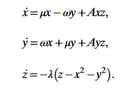
Here, x,y and z are the first, second and shift mode respectively. The evolution of this system of equations is shown in the figure below, as well as a representation of the different modes. The indicated limit cycle describes the case where the Von Karman vortex street is fully developed and the mean field alternates between the first and second mode, with a strong presence of the shift mode. Quite remarkably, the full complexity of the original system can be compressed almost completely into a 3D space! This is the power of the POD method and, if you will, the power of the scientist.

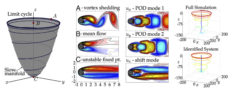
—‘Discovering Governing Equations from Data by Sparse Identification of Nonlinear Dynamical Systems’ [1]

A time series of these three coordinates was given to SINDy and again the original dynamics were recovered very accurately. Interestingly, it took the scientific community over 15 years to reach consensus on the theoretical solution regarding this problem. Here, with the help of SINDy and some background knowledge on the system, the solution was recovered right away.

Specifics of SINDy

Optimization and sparseness

So far, my focus has been on intuitively introducing the method, without going into too much technical detail. By now, you hopefully have some intuition on how the technique approaches model discovery. Before going further and talking about extensions and updates to SINDy, there are two burning questions that perhaps require answering: how does SINDy actually optimize, and how does one include the requirement of sparseness?

Both of these questions are closely related and the key lies in the specific form of the loss function. Everyone who is familiar with machine learning should have a pretty good idea of what a loss function is and how it forms a central part of the optimization. SINDy uses a pointwise l₂ loss between the ground truth and prediction (as is very standard for regression problems), but extends this with a sparsity promoting term to reduce the complexity. In essence, the loss function corresponds to the following:

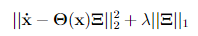
The first term makes sure the regression is accurate, while the second term penalizes the presence of nonzero terms in the coefficient matrix (the more nonzero terms, the higher the norm of this matrix). The form shown here corresponds to the least absolute shrinkage and selection operator (LASSO), basically providing l₁ regularization. In practice however, this is not what is applied in SINDy, as it can become really expensive to calculate for large datasets. Instead, a so-called sequential thresholded least-squares method is used. In this method, terms of the coefficient matrix that are below a certain threshold are set to zero and removed/made inactive at fixed intervals in the training, after which the least-squares regression optimization is continued. This is done until sufficient sparsity is achieved and the training finishes. The resulting solution is very similar to what the loss function above, with LASSO, would lead to.

The $\lambda$ parameter as well as the actual threshold value for deletion give the needed flexibility for the SINDy algorithm, specifically how strong we want to regularize the problem.

The function library

At this point, you might still be bugged by a very apparent flaw. “Alright, we should use our prior knowledge on the system to optimize how we approach the problem, but how do we create a perfect library?” The question of what terms we should include is a tricky one to answer, and it is closely connected to the problem of having a right coordinate system. The algorithm carries at its heart the assumption of sparsity, but this is likely only true in an ideal basis of the right coordinates. If the dynamics exhibit periodicity, we cannot expect a library of polynomials to provide good results, but how do we recognize periodicity if we monitor the wrong coordinates? This problem wasn’t addressed in the first paper on the subject and felt like a very strong limitation to the universal applicability of the algorithm. Luckily, the authors have been quite busy these past few years and a follow-up paper might provide a way out.

Finding coordinates

‘Data-Driven Discovery of Coordinates and Governing Equations’ [2] explores how we can find the appropriate coordinates in which to describe our system. As stated before, this was one of the main missing elements of the original algorithm and it might be as crucial as finding the actual model. Many of the great breakthroughs in history were facilitated first by the discovery of the right coordinates. Think of the geocentric versus heliocentric model of the solar system and how this revolutionized our understanding and the models, as a prime example.

In this paper, a method is explored where the algorithm simultaneously learns an adequate coordinate system and also finds the model dynamics. It does so by extending the original model with an autoencoder and adding extra terms to the loss function, in order to guarantee convergence.

Autoencoders

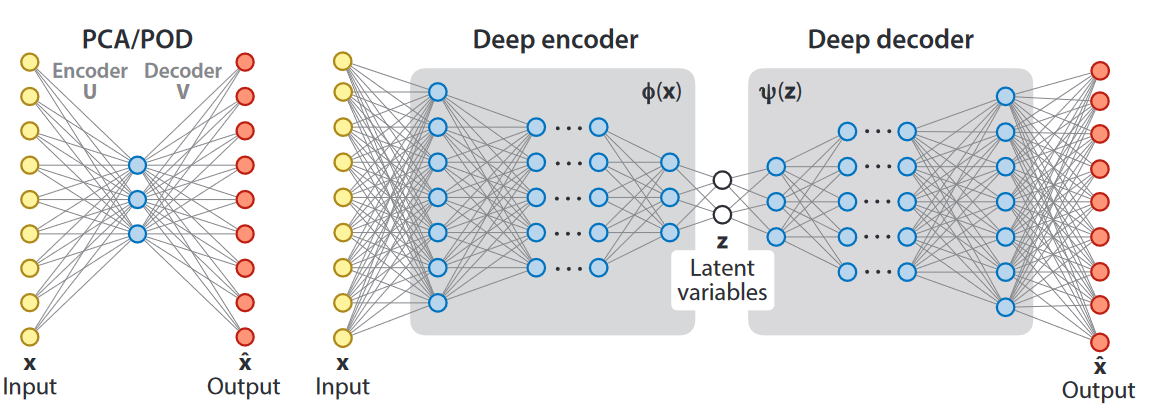
Autoencoders are a type of neural network where the input and output layers are identical in shape, and the -usual- goal is to reproduce the output as accurately as possible while having a limited number of hidden nodes. First, the encoder compresses the input data into the lower-dimensional middle layer. Then, a decoder has to reconstruct the input again from this information. In this sense, autoencoders are like a nonlinear extension of PCA/POD where the data are transformed to a new coordinate system in the restricted hidden layer. The nonlinearity is imposed by having nonlinear activation functions in between the layers and by preferably having multiple layers. This results in a deep autoencoder (see below) and is exactly the structure that is used here for coordinate discovery.

The updated algorithm

To perform the joint optimization task of finding coordinates and a model, the SINDy algorithm is applied to the reduced coordinates z(t) = $\phi$(x(t)) which are learned simultaniously. The model for the dynamics in z will again be sparse.

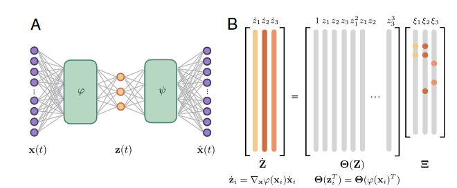
—‘Data-Driven Discovery of Coordinates and Governing Equations’ [2]

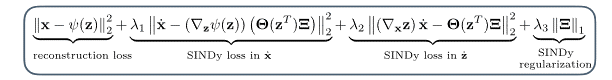
The schematic representation above shows the updated version of the SINDy algorithm, as well as the new loss function. The last two terms in this loss function are essentially the same ones as encountered in the original model, but now the two first terms have to be added to ensure correct convergence. The reconstruction loss makes sure that the autoencoder performs as expected for every timeframe, reproducing a close fit to the input data. The ‘SINDy loss in $\dot x$’ term serves the same purpose as the one in $\dot z$ and is just added to verify that the correct dynamics in z also translate to the correct ones in the physical/measured coordinates. Intuitively, one would expect this to always be the case, but it turns out that reality is a little more intricate, hence the extra term.

As the dimensionality of the reduced layer is usually much lower than that of the input, z will be the result of some nonlinear embedding. The actual dimension is a hyperparameter that is to be specified prior to training. This is one of the limitations of the algorithm: we either have to try multiple values to find the optimum, have prior knowledge on the dimensionality, or make a trade-off between simplicity and accuracy.

As a “bonus” though, the fact that we are now solving both the problems of finding coordinates and model optimization at the same time might make the second fundamental problem we had redundant. It is feasible that a nonlinear embedding that is learned on the spot can allow for the dynamics to be described by much simpler terms, perhaps even linear terms or simple period ones. So, while the construction of a good function library is still a requirement, it might be a bit less restrictive once we have the flexibility of the embedding.

Examples

—‘Data-Driven Discovery of Coordinates and Governing Equations’ [2]

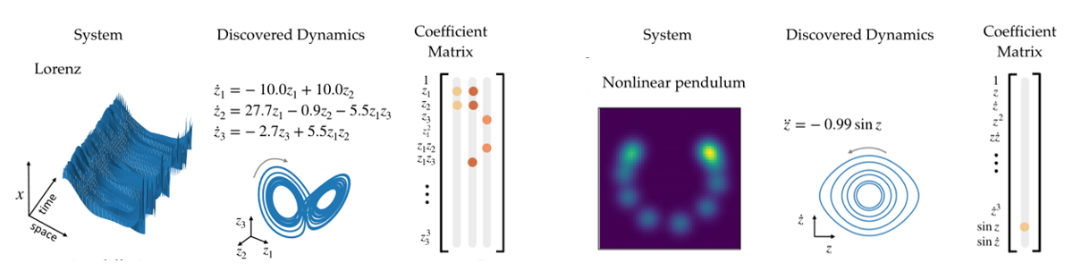
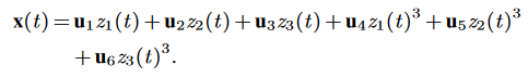
To showcase the workings of the extended algorithm, two of the examples discussed in the paper are shown in the figure above. The first problem is quite ‘synthetic’: the Lorenz system from before is used as the hidden underlying dynamics for a new system: a nonlinear combination of the three coordinates z_1,2,3(t) with 6 fixed spatial modes u_n is made to create input data x(t) that has 128 spatial values and evolves over time:

The goal of the autoencoder is to ‘learn’ this nonlinear transformation that has been applied and to rediscover the z(t) coordinates, as they allow for the system dynamics to be described in a very sparse and low-dimensional fashion. Up to arbitrary scaling and an unsignificant coordinate transformation, the original system is recovered remarkably well, as can be verified by comparing the result with the original Lorenz system.

The second example is that of a nonlinear pendulum. The input is a simulated video of a nonlinear pendulum with a 2D Gaussian as the moving object, with the peak corresponding to the centre of mass. Every frame is high dimensional, despite the fact that the dynamics can be described simply in terms of the angle of the pendulum. Again, some prior information is implemented in the sense that the restricted space consists of only one coordinate. Even then, the algorithm succeeds in discovering the correct dynamics (most of the time, according to the authors the same experiment was repeated multiple times). Notably, this example has a second order ODE as underlying dynamics. The first order time derivative was also computed and relevant terms were included in the function library for this case. The approach remains essentially the same, but it seems that SINDy has no real problems with this extension.

Further improvements - PDE-FIND

As a last addition -and without going into much detail-, I will quickly present the main results of a third connected paper. The main reason for this is just to emphasize once again, that the research is still very active and updates, improvements and new ideas are constantly popping up.

This third paper, ‘Data-Driven Discovery of Partial Differential Equations’ [3], addresses some of the apparent limitations of the previous work:

• Learning the right coordinates can be really expensive on big input spaces and the algorithm stuggles with high dimensional data
• Full information in space and time is often not available in experiments
• So far, the work has been resricted to ODE’s
• The training data doesn’t always cover the full dynamic range

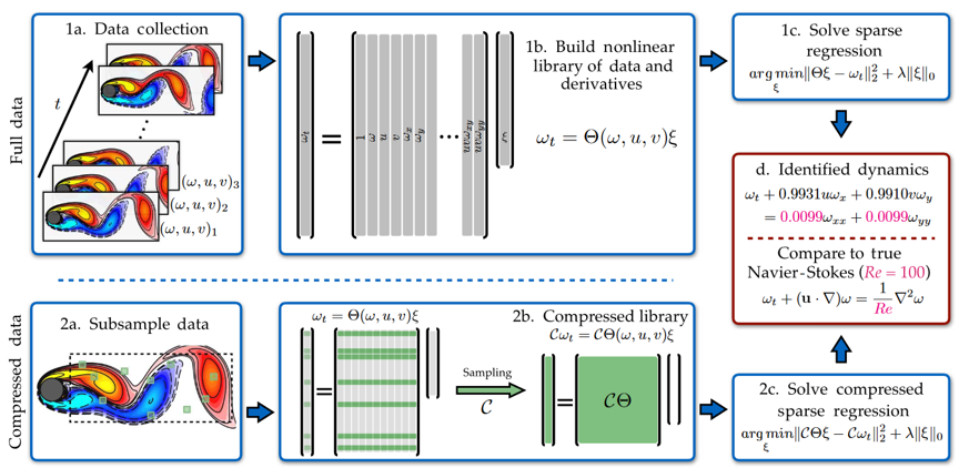
The first problem was overcome previously by dimensionality reduction methods like POD. This approach, however, requires manipulation by the user and implies an extra loss of information. The algorithm proposed in this paper, called PDE-FIND, proposes a different approach. In fact, it tackles both the first and second problem at the same time! It does so by being able to use subsampled data without any notable loss of accuracy in its prediction. The schematic structure is shown in the figure below. Using the data from just a few points (sensors in an experiment), either Lagrangian or Eulerian, the algorithm still manages to come up with the correct dynamical system.

—‘Data-Driven Discovery of Partial Differential Equations’ [3]

As can be seen, the subsampling essentially corresponds to using only a fraction of the rows (subsampling in time) and columns (subsampling in space) of the original matrix problem.

For the third problem, even though PDE-FIND uses only subsampled data at specific points, it needs some information in the direct neighbourhood of these points to approximate spatial derivatives as well. Whereas the previous algorithms focused on only temporal derivatives, this work was able to solve very general PDE’s and spatiotemporal problems.

As a nice example that also covers the fourth problem stated, the algorithm was used to retrieve the Korteweg-de Vries equation: u_t + 6uu_x + u_xxx = 0. This wave equation is highly nonlinear with third order spatial derivative terms and proapagation speeds proportional to the amplitude of wave solitons. When only a singly time series is given to train on (one traveling wave), the dynamics would be indistinguishable from just a one-way wave equation u_t +cu_x =0. The figure below shows how unlike previously, PDE-FIND can use input data with multiple initial amplitude solitons to disambigue between the different dynamical systems. The principle is shown below.

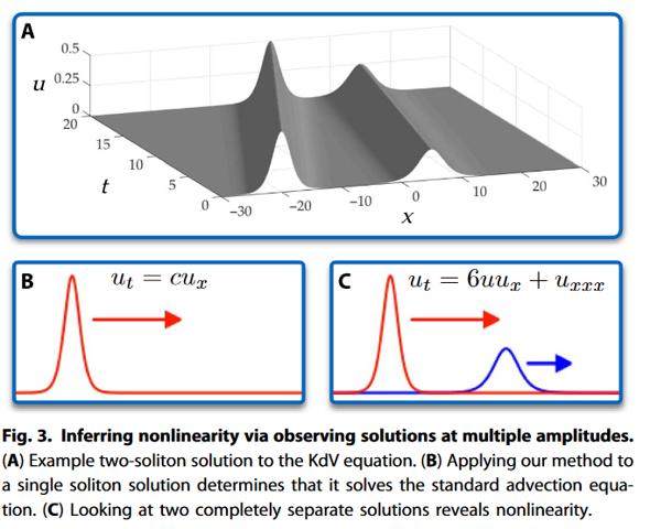
—‘Data-Driven Discovery of Partial Differential Equations’ [3]

Conclusions

SINDy may still be in its infancy, but it is clear that the method is very promising. The application of machine learning in science is one of the fastest growing fields of research, with successes and breakthroughs in many areas. The idea behind the SINDy algorithm gives us a unique opportunity to discover and investigate systems that were beyond our reach before and it has one major advantage: SINDy is interpretable and -at least to some extent- extrapolatable. This is in my opinion the most valuable aspect of this research. It can deal with noise, incomplete data, general PDE’s, high-dimensional data and much more, but in an environment dominated by black-box surrogate models and blind machine learning, the approach taken with SINDy might be the way for science to move forward. Not swallowed by or replaced by the computational power of the future, but augmented by it.

Bibliography

• [1] Brunton, Steven L., Joshua L. Proctor, and J. Nathan Kutz. ‘Discovering Governing Equations from Data by Sparse Identification of Nonlinear Dynamical Systems’. Proceedings of the National Academy of Sciences 113, no. 15 (12 April 2016): 3932–37. https://doi.org/10.1073/pnas.1517384113.

• [2] Champion, Kathleen, Bethany Lusch, J. Nathan Kutz, and Steven L. Brunton. ‘Data-Driven Discovery of Coordinates and Governing Equations’. Proceedings of the National Academy of Sciences 116, no. 45 (5 November 2019): 22445–51. https://doi.org/10.1073/pnas.1906995116.

• [3] Rudy, Samuel H., Steven L. Brunton, Joshua L. Proctor, and J. Nathan Kutz. ‘Data-Driven Discovery of Partial Differential Equations’. Science Advances 3, no. 4 (7 April 2017): e1602614. https://doi.org/10.1126/sciadv.1602614.